Single timestep

Illustrates setting up a simulation and solving at a single time step

from platform import release
import re
import numpy as np
import xcell as xc
import matplotlib.pyplot as plt

Set simulation preferences

# Misc parameters
study_path = "/dev/null"

# options = uniform, adaptive
meshtype = "adaptive"

max_depth = 10  # Maximum successive splits allowed for octree mesh
nX = 10  # Number of elements along an axis for a uniform mesh

# options: Admittance, Face, FEM
element_type = "Admittance"
dual = True
regularize = False

# options: analytical, ground
boundaryType = "ground"

fixedSource = False  # otherwise, simulate current injection

Run simulation

xmax = 1e-4  # domain boundary
rElec = 1e-6  # center source radius

sigma = np.ones(3)

bbox = np.append(-xmax * np.ones(3), xmax * np.ones(3))
study = xc.Study(study_path, bbox)

setup = study.new_simulation()
setup.mesh.element_type = element_type
setup.meshtype = meshtype

geo = xc.geometry.Sphere(center=np.zeros(3), radius=rElec)

if fixedSource:
    setup.add_voltage_source(xc.signals.Signal(1), geo)
    srcMag = 1.0
    srcType = "Voltage"
else:
    srcMag = 4 * np.pi * sigma[0] * rElec
    setup.add_current_source(xc.signals.Signal(srcMag), geo)
    srcType = "Current"

if meshtype == "uniform":
    setup.make_uniform_grid(nX)
    print("uniform, %d per axis" % nX)
else:
    setup.make_adaptive_grid(
        ref_pts=np.zeros((1, 3)),
        max_depth=np.array(max_depth, ndmin=1),
        min_l0_function=xc.general_metric,
        # coefs=np.array(2**(-0.2*max_depth), ndmin=1))
        coefs=np.array(0.2, ndmin=1),
    )

if boundaryType == "analytical":
    boundary_function = None
else:

    def boundary_function(coord):
        r = np.linalg.norm(coord)
        return rElec / (r * np.pi * 4)


setup.finalize_mesh()

setup.set_boundary_nodes(boundary_function, sigma=1)

v = setup.solve()
setup.apply_transforms()


setup.getMemUsage(True)
setup.print_total_time()

setup.start_timing("Estimate error")
# srcMag,srcType,showPlots=showGraphs)
errEst, arErr, _, _, _ = setup.calculate_errors()
print("error: %g" % errEst)
setup.log_time()

bnd = setup.mesh.bbox[[0, 3, 2, 4]]

927.842 Mb used
        Total time: 2.15392s [CPU], 1.45783s [Wall]
error: 0.217408

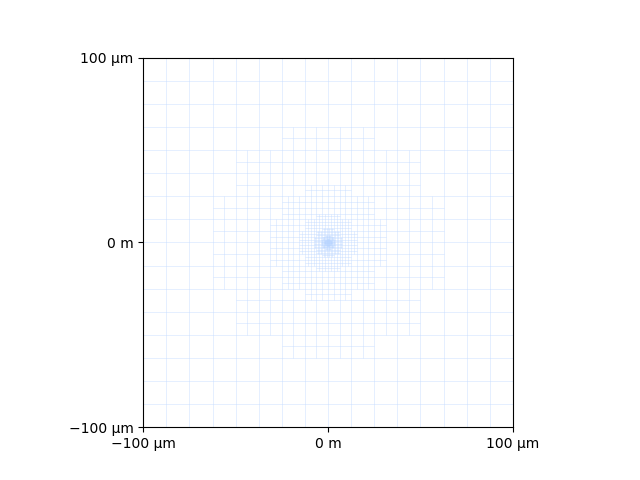
ax = plt.figure().add_subplot()
xc.visualizers.format_xy_axis(ax, bnd)
arr = xc.visualizers.resample_plane(ax, setup)

colormap, color_norm = xc.visualizers.get_cmap(arr.ravel(), forceBipolar=True)
xc.visualizers.patchwork_image(ax, [arr], colormap, color_norm, extent=bnd)

_, _, edge_points = setup.get_elements_in_plane()
xc.visualizers.show_2d_edges(ax, edge_points)

<matplotlib.collections.LineCollection object at 0x2ccf7af10>

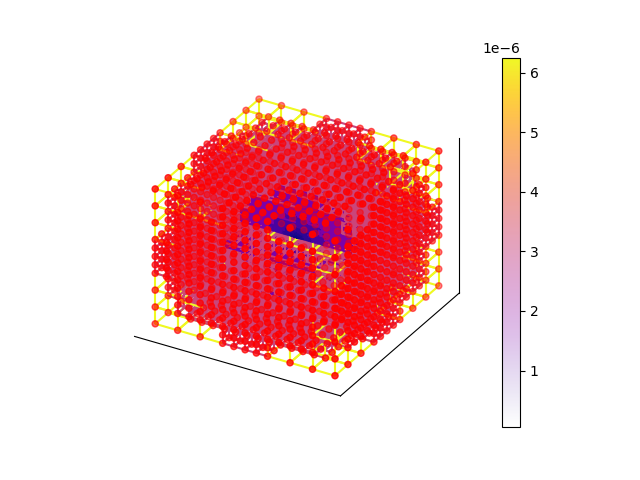
TOPOLOGY/connectivity

ax = xc.visualizers.show_mesh(setup)
ax.set_xticks([])
ax.set_yticks([])
ax.set_zticks([])
ghost = (0.0, 0.0, 0.0, 0.0)
ax.xaxis.set_pane_color(ghost)
ax.yaxis.set_pane_color(ghost)
ax.zaxis.set_pane_color(ghost)


xc.visualizers.show_3d_edges(ax, setup.mesh.node_coords, setup.edges, setup.conductances)

bnodes = setup.mesh.get_boundary_nodes()
xc.visualizers.show_3d_nodes(ax, setup.mesh.node_coords[bnodes], node_values=np.ones_like(bnodes), colors="r")

<mpl_toolkits.mplot3d.art3d.Path3DCollection object at 0x2ccfde910>

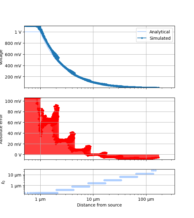
SliceSet

# sphinx_gallery_thumbnail_number = 4
img = xc.visualizers.SliceSet(plt.figure(), study)
img.add_simulation_data(setup, append=True)
_ = img.get_artists(0)

ErrorGraph

ptr = xc.visualizers.ErrorGraph(plt.figure(), study)
ptr.prefs["universalPts"] = True
pdata = ptr.add_simulation_data(setup)
_ = ptr.get_artists(0, pdata)

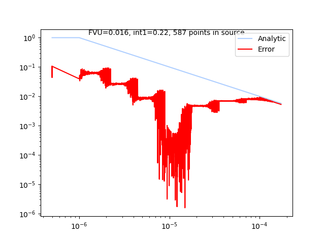
LogError

P = xc.visualizers.LogError(None, study)
P.add_simulation_data(setup, True)
_ = P.get_artists(0)